Pinch Analysis is an energy integration methodology widely used in chemical and petrochemical processes. Its main goal is to reduce the consumption of external utilities, such as steam and cooling water, by maximizing energy recovery within the plant itself. The technique emerged in the 1970s and became a fundamental tool in the design of heat exchanger systems.
The central concept of Pinch Analysis is identifying the so-called “pinch point”, which corresponds to the system’s thermal bottleneck. This point sets the limits of heat recovery and guides the design rules that must be followed to ensure minimum utility use. The methodology applies to any system in which hot streams, which need to be cooled, coexist with cold streams, which need to be heated.
The first step in applying Pinch Analysis is to identify the process streams. For each stream, the inlet temperature, outlet temperature and heat capacity flow rate (mass flow rate times specific heat, ṁ·Cp) must be known. Next, the minimum allowable temperature difference between streams in heat exchangers (ΔTmin, or approach) is defined, usually between 10 °C and 20 °C, which directly affects the balance between capital and operating costs.
To illustrate, consider an example using the streams shown in Table 1. For this system, we will assume ΔTmin = 20 °C.
Table 1 – Process streams
| No. | Stream Name | Stream type | Supply Temperature | Target Temperature | ṁ·Cp kW / K |
Heat Load kW |
| 1 | CE | Hot | 120 | 30 | 993 | 89373 |
| 2 | VN | Hot | 95 | 50 | 1317 | 59273 |
| 3 | CO | Hot | 95 | 50 | 153 | 6878 |
| 4 | VI | Hot | 34 | 29 | 9333 | 46667 |
| 5 | CP | Cold | 30 | 105 | -736 | -55200 |
| 6 | CS | Cold | 48 | 105 | -703 | -40082 |
| 7 | CC | Cold | 95 | 127 | -1496 | -47875 |
| 8 | DES | Cold | 25 | 120 | -29 | -2771 |
From these data, the composite curves are built. To do so, all hot streams are shifted by -ΔTmin/2, while cold streams are shifted by +ΔTmin/2. Figure 1 shows these streams in a T×ΔH diagram. In this representation, the x-axis represents the heat load and the slope of the curves represents the heat capacity flow rate of each stream.
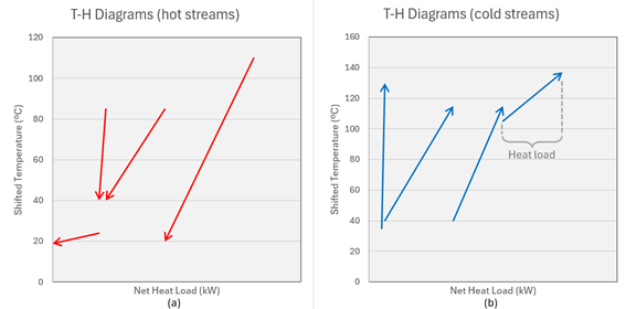
Figure 1 – Temperature vs. enthalpy change diagram. (a) shows the hot streams plotted separately on a temperature-heat diagram. (b) shows the cold streams plotted separately on a temperature-duty diagram.
The composite curve is built simply by adding up the enthalpy changes of the individual streams within each temperature interval. The sum of the heat capacity flow rates in each temperature range defines the slope of the curves. The point where the curves meet is the pinch point, which marks the boundary between the upper region (above the pinch) and the lower region (below the pinch).
Figure 2 (a) shows the result of this procedure for the proposed numerical example. The red curve represents the composite of the hot streams and the blue curve that of the cold streams. The point where they come closest is the pinch point, from which the design rules are defined. Figure 2 (b) shows the curve at actual temperature, +ΔTmin/2 for the cold stream and –ΔTmin/2 for the hot stream. The distance between the curves is ΔTmin (approach), set at the start of the calculations. Above the pinch, cooling utilities should not be used, and below it, heating utilities should not be used.
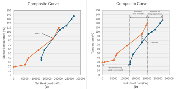
Figura 2 – Composite curve. (a) shifted temperature. (b) actual temperature
This result makes it possible to quantify minimum utility consumption. The offset between the hot and cold curves at the highest temperatures shows the minimum amount of steam needed to heat the cold streams. Likewise, the difference between the start of the hot curve and the cold curve at lower temperatures defines the minimum cooling water requirement. Pinch Analysis therefore not only indicates where to install heat exchangers but also provides the system’s thermodynamic limits.
The grand composite curve shown in Figure 3 is built by plotting the heat load difference between the hot and cold composite curves of Figure 2 (a) as a function of temperature. It provides a graphical representation of heat flow through the process — from the hot utility to the parts of the process above the pinch, and from the process below the pinch to the cold utility.
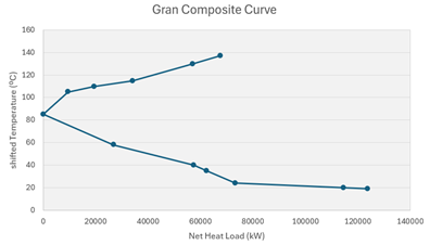
Figure 3 – Grand Composite Curve
A significant advantage of the methodology is that it is not limited to optimizing existing processes; it can also be used at the conceptual design stage of new units. Engineers can thus predict energy demand before equipment is even installed, reducing operating costs over the plant’s entire service life. The analysis can also be extended to include utility integration, cogeneration and even mass balances.
It is important to note that practical application of Pinch Analysis must take economic and operational aspects into account. In some cases, even if theory points to maximum integration, layout, safety or reliability constraints may justify using additional utilities. The technique should therefore be seen as a decision-support tool rather than a one-size-fits-all solution.
In short, Pinch Analysis enables significant gains in energy efficiency. By identifying heat recovery limits and guiding the optimal allocation of exchangers, it contributes directly to industrial sustainability, reducing greenhouse gas emissions and resource consumption. Its use is highly recommended in energy-intensive sectors such as agribusiness, petrochemicals, pulp and paper, and food.
References
- Linnhoff, B., & Hindmarsh, E. (1983). The pinch design method for heat exchanger networks. Chemical Engineering Science, 38(5), 745–763.
- Kemp, I. C. (2007). Pinch Analysis and Process Integration: A User Guide on Process Integration for the Efficient Use of Energy. Butterworth-Heinemann.
- Smith, R. (2016). Chemical Process Design and Integration. Wiley.
Rubens Eliseu Nicula De Castro
Specialist Engineer – A1 Engenharia.
- Chemical Engineer;
- PhD in Chemical Engineering;
- MBA in Project Management.